The dynamic time warping method is one technique used for speech recognition. The first step is to properly detect the endpoints of each word using Rabiner & Sambur’s endpoint detection method. This method takes into account both energy level per frame, and number of endpoints per frame, due to low energy level of fricatives. Once endpoint detection takes place, the individual words are split into frames, and then split into 17 critical bands using a filter bank. The energy level for each band is used as an attribute in the dynamic time warping matrix. Next, the available recording data was split into training and testing sets. The local distance matrix is created with the training set on the horizontal axis and the testing set on the vertical axis. Each value in the matrix consists of the difference between the ith instance in the training set and jth instance in the testing set, using city block distance to find the distance for all attributes. Next, the accumulated distance matrix is formed by finding the shortest path from the top left corner to bottom left corner. For a single testing example, an LMD and AMD are formed for each word in the database, with the shortest distance in the bottom of the right hand corner of the AMD indicating the correct word.
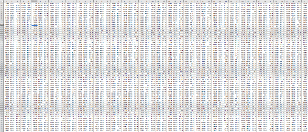
LMD:
AMD: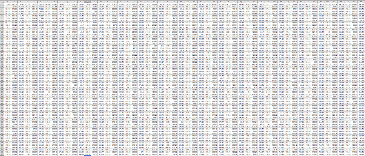
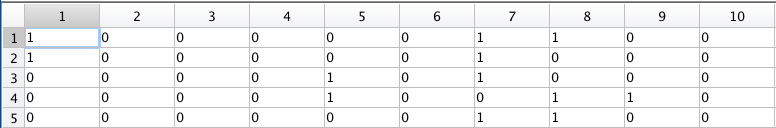
For the ten words in the set, there are 5 instances of each word. Cross validation is done where each of the words in the set is used as a test and compared against the other data. This leads to a 10×5 confusion matrix consisting of logical values of whether or not the word was correctly detected.
With non-noisy audio files, the total accuracy was 24%. There were several potential points of error, most importantly being that the thresholds in the end-point detection needed to be adjusted manually.
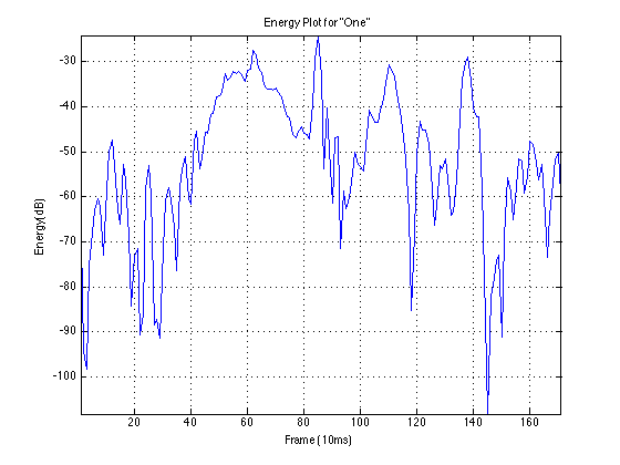
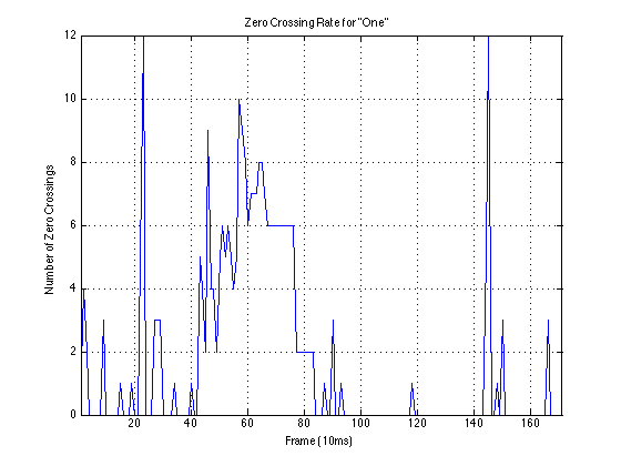
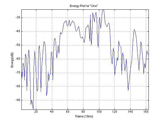
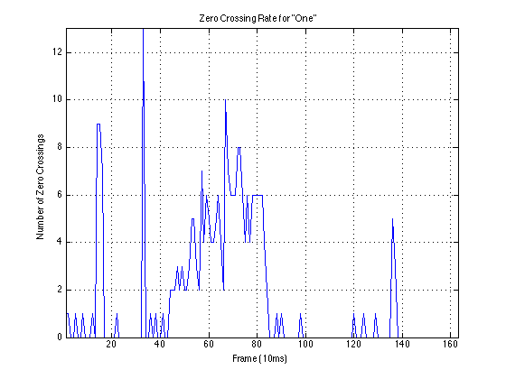
Example Data: “One”
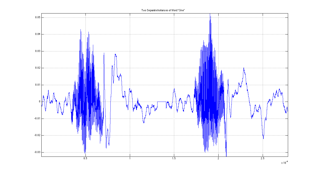
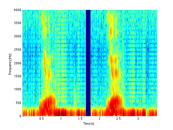
First Instance:
Second Instance:
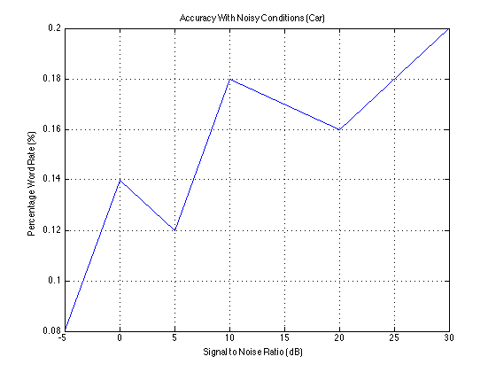
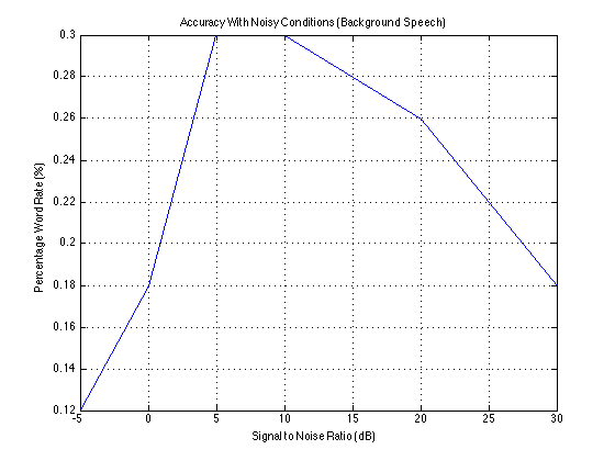
To test the algorithm’s functionality in noisy circumstances, different levels of noise from (a) an automobile and (b) random background talking were added to the speech samples. The following graphs plot accuracy against signal to noise ratio. The car noise behaves as expected, with accuracy higher as the signal to noise ratio increases. While the speech sample accuracy increases briefly, the accuracy again drops off.
 Download Code and Audio